OpenLogger Origins: The Beginning

Over the past few months we’ve been excitedly discussing the launch of the OpenLogger on Crowd Supply, and how the OpenLogger came to be. OpenLogger was first conceived by one of our engineers with a passion to push the boundaries of ADC and DAC technology with the PIC32MZ, and when we launched the OpenSco pe on Kickstarter, one of our stretch goals was to add Data Logging functionality to the two Analog inputs. In reaching this goal and adding this functionality, we discovered the potential that the hardware had when focused on Data logging. Through this discovering, and pushing the functionality of the technology, OpenLogger was born.

To highlight the differences between the OpenScope and OpenLogger we’ve asked Keith, the head engineer on the project, to share his take and experience. In the next couple of posts, he will discuss some background on oscilloscopes, and data loggers, and some of the technical challenges and discoveries of the OpenScope and OpenLogger.

What was the background of the project?

The OpenScope was introduced as an MCU based 6.25MS/s oscilloscope as part of a Kickstarter campaign last year. As a stretch goal, 2 – 50kS/s data logging channels were implemented using the analog input channels. At first glance, this would seem to be an easy feature to add as the much faster oscilloscope channels already existed. However, to my surprise, data logging is a very different and much more difficult instrument to implement than an oscilloscope. Implementing both the oscilloscope and data logging functionality on the same OpenScope hardware provided for a uniquely identifiable contrast of the two instruments.

Can you tell me about the oscilloscope?

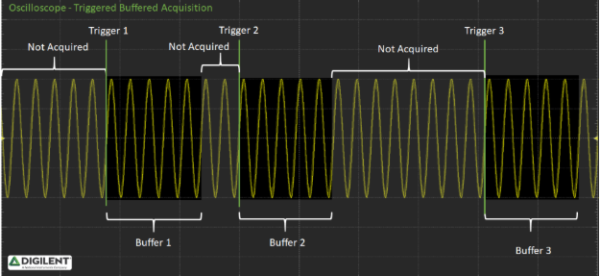
Oscilloscopes perform triggered buffered acquisition meaning a finite amount of data is acquired in response to a ‘trigger’ event. Between trigger events data may not be sampled.

An oscilloscope trace is implemented by starting the ADC conversions at some, typically, high sample rate. The intent is to capture as much detail of the signal a possible. To do this, almost no processing of the raw ADC data can be done while capturing the data. When the ADC conversion is complete, the raw data is saved in a buffer to be post-processed later. In the case of the OpenScope, a sample rate timer is used to initiate ADC conversions. On the ADC completion event, a DMA transfer moves the raw ADC data to memory. The DMA is configured to fill the DMA ring buffer, automatically wrapping back to the beginning of the buffer when full and continuing to overwrite the oldest data. This continues until a trigger event is sensed. Once the trigger is detected, the DMA continues to transfer post trigger data until a time out event stops the ADC conversion. When done, the DMA ring buffer has both pre and post trigger data (assuming there is no trigger offset). The DMA hardware is limited to a maximum buffer size of 64kB, and at 2 bytes per sample, can hold a total of 32k samples.

Since the DMA can only hold 32k samples, at 6.25MS/s that is only about 5 milliseconds of pre and post triggered data. Once all of the data for the trace is collected, the data is post processed to convert the raw ADC values into actual voltages. Then the data is reported to Waveforms Live for display. If the OpenScope is configured to “run” as opposed to a “single” trace, WaveForms Live automatically reissues another single trace command after displaying the previous trace; this is repeated simulating a trace “run”. The actual number of traces displayed per second through WaveForms Live is highly variable on how fast you are sampling, how big the sample buffer is (maximum of 32k samples), how fast the communication is between the OpenScope and WaveForms Live, and how fast the browser can draw the signal on the display.

Consolidating the process, here are the steps taken for a trace:

1. Configure the offset, gain and other parameters

2. Start sampling

3. Start capturing raw ADC data into a ring buffer

4. Enable the trigger

5. Wait for the trigger

6. Collect post trigger data into the ring buffer

7. Stop capturing data

8. Post process the raw ADC data to voltages

9. Transfer the voltages to WaveForms Live

10. Display the voltages on the display

11. Start all over again

How about the data logging?

Unlike an oscilloscope trace, data logging is a continuous process. There is no trigger, you just start logging and you take samples at a regular rate; continuously, non-stop, until you decide to stop logging data. Seems simple enough right? But wait, how big is the ring buffer? When do you post process the data? When do you transfer the data to the user interface? In a nutshell the data must be processed, saved, transferred, and displayed WHILE continuing to sample, without missing a single sample. Except for the trigger mechanism, all the oscilloscope steps must occur concurrently for data logging; not sequentially.

Now, we do get some help. Typically, data logging occurs at a much slower sample rate than an oscilloscope but typically we expect more bits of resolution. The trade-off is, slower sample rate, but higher precision gapless data. However, since data logging is a continuous process, very little of the implementation of an oscilloscope can be used to implement data logging. The relentless, continuous nature of data logging brings on complications of where to store or how to display the data, and the requirement that not one sample can be lost over a potentially very long period of time. Consider some of the extremes, at 50kS/s; 1 day of data would consume over 4 billion samples, of which you can miss none. If we are going to log biometrics, or manufacturing data, or environmental conditions; the sample rate may be very slow but would be taken over days, months, even years. At a sample rate of 1 sample per day for a year, that is only 365 samples; yet, you must be up and running without crashing for a year (how many electronic devices run for year without crashing?).

Here are some considerations for data logging:

* Continuous processing of ADC data to voltages, on the fly, while sampling is occurring.

* The requirement to record (store) every sample over long periods of time potentially resulting in very large sample sets.

* The requirement that the system stays operational for extremely long periods of time; without crashing or rebooting.

* Sampling clocks and timing must be accurate over long periods of time.

o Consider a 25ppm clock, that can be off by as much as 2 seconds a day or 730 seconds per year (12 hours off in a year).

o A simple clock will not work, it must be either very accurate, or get periodic updates to correct for error.

* Oscilloscopes sample at higher rates and lower precision, data logging sample at lower rates but higher precision:

o The analog input circuit for oscilloscopes must be designed for a higher bandwidth, whereas data logging should be designed for a lower bandwidth.

o Lower samples rates allows for less noise through better filtering and therefore better precision.

o Lower bandwidth potentially allow for less expensive analog components.

o For example, the OpenScope analog bandwidth is 2.5MHz whereas the OpenLogger is designed with a 50kHz analog bandwidth

* Because a user may not watch every sample, it would be ideal if the UI (WaveForms Live) was able to disconnect and reconnect as well as resynchronize without interfering with ongoing sampling.

* While the system is sampling, it would be ideal if the UI was able to query and display current as well as past data.

o This requires reading past data from storage (say an SD card) while concurrently saving current data; without interfering with sampling

If you have any more questions about the OpenLogger stay tuned for next week where we will release the next post in this series or feel free to inquire in the comments below!

+3

0